Sorting
Feb 3, 2015 · 9 minute readMost programming languages have an extremely efficient, optimized in nearly all cases, built in sorting algorithm that’s a simple function call away. Practically, this removes the need to spend much time contemplating the implementation, efficiencies, and tradeoffs behind the many existing ways to sort, and instead focus on the “actual problem”. Nonetheless, it is informative to walk through the basics of sorting in order to gain a more comprehensive understanding of the current state of the art algorithms.
Before diving into specifics, there are 3 things to note about sorting in general.
- All general purpose sorting algorithms fall into the category of comparison sorts, meaning that they depend solely on the ability to compare any two elements and determine which one should come first in the sorted result, and the ability to rearrange elements.
- Sorting algorithms can either use additional buffer space to do their work, or perform the sort “in place”. In place sorts use constant (or occasionally logarithmic) additional storage space, as opposed to
O(n)or more additional memory via a working buffer for regular implementations. - All comparison based sorting algorithms require at least linearithmic asymptotic running time.
The comparison sorting properties are codified in an interface like the following:
type ComparisonSortInterface interface {
    // Less reports whether the element with
    // index i should sort before the element with index j.
    Less(i, j int) bool
    // Swap swaps the elements with indexes i and j.
    Swap(i, j int)
}
All the comparison based sorting implementations below will depend solely on that interface.
Selection Sort
Upon learning of the “sorting problem”, this is the algorithm that many students initially devise. Essentially, the idea is to select the smallest element, and move it to the front of the input collection. Then, select the next smallest element, and move it to the second place in the collection, continuing in this manner until the entire collection is sorted. In code, it looks like the following:
func SelectionSort(data sort.Interface, a, b int) {
    if b <= a {
        return
    }
    smallestElementIdx := a
    for i := a + 1; i < b; i++ {
        if data.Less(i, smallestElementIdx) {
            smallestElementIdx = i
        }
    }
    data.Swap(a, smallestElementIdx)

    SelectionSort(data, a+1, b)
}
Unfortunately, this algorithm is not very efficient,
with a best and worst case time complexity of O(n^2).
As written, the algorithm performs the sort in place,
but since it is implemented recursively,
and Go does not optimize tail recursion,
it has a linear memory requirement via the call stack.
Go is efficient enough that the recursive implementation does not matter in practice
(the sort becomes impractically slow due to the quadratic runtime before it approaches the stack space limit),
and I like the elegance of the recursion more than an extra loop, so I left it as is.
Bubble Sort

This is another basic sorting algorithm. The idea is to bubble larger elements towards the end of the list, performing this bubbling until the entire collection is sorted. In code:
func BubbleSort(data sort.Interface, a, b int) {
    performedSwap := false
    for i := a + 1; i < b; i++ {
        if data.Less(i, i-1) {
            performedSwap = true
            data.Swap(i, i-1)
        }
    }

    if performedSwap {
        // we know that the largest element is at the end, now sort the rest of the list
        BubbleSort(data, a, b-1)
    }
    // if no swap was performed, the list is sorted
    return
}
This algorithm has similar performance characteristics to the Selection Sort above,
but with the nicety that if the collection is already sorted,
it finishes in O(n) time.
Insertion Sort

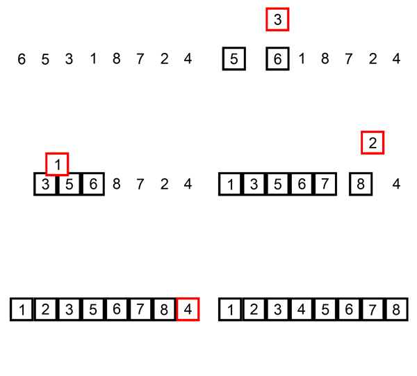
Insertion sort works by going through the collection, and inserting each element into a sorted version of the collection, until the entire thing is sorted. Insertion sort is usually performed in place, moving elements around in the collection to keep the sorted version at the front.
func InsertionSort(data sort.Interface, a, b int) {
    for i := a + 1; i < b; i++ {
        for j := i; j > a && data.Less(j, j-1); j-- {
            data.Swap(j, j-1)
        }
    }
}
Efficiency is on par with the first 2 algorithms,
with a best and worst case of O(n^2).
Note that this particular implementation is in-place,
and eschews recursion, therefore using no additional memory.
Merge Sort

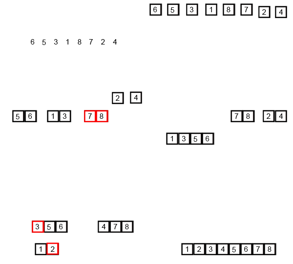
While the first 3 sorts were fairly simple and straightforward, this one is more complex. Accompanying its complexity, however, is better runtime efficiency. Merge sort works by recursively merging sorted subcollections of the input collection. Effectively, this means that it takes the input collection, and breaks it down into sub-collections that are sorted (the base case being a collection with just 1 element, which is sorted by default). Subsequently, these sub-collections are merged back together, maintaining the sorted order, resulting in a larger, sorted sub-collection. Eventually, this process results in the entire collection being sorted.
func MergeSort(data sort.Interface, a, b int) {
    if b-a < 2 {
        return
    }

    mid := a + (b-a)/2
    MergeSort(data, a, mid)
    MergeSort(data, mid, b)
    merge(data, a, mid, b)
}

// Merges (in place) the two sorted logical collections represented by the indices
// [a, m) and [m, b) of the input data collection. The result is a sorted logical
// collection that extends from a to b.
func merge(data sort.Interface, a, m, b int) {
    // check if the two collections are already sorted
    if data.Less(m-1, m) {
        return
    }

    i, j := a, m
    for i < j && j < b {
        if data.Less(i, j) {
            i++
        } else {
            j++
            shiftRight(data, i, j)
            // update i pointer to take the shift into account
            i++
        }
    }
    // whatever remains is already in the right place
}

// Shifts the data elements in the collection slice data[a,b) to the right
// by one element, with wraparound, meaning the last element in the slice is now
// the first element
func shiftRight(data sort.Interface, a, b int) {
    for i := b - 1; i > a; i-- {
        data.Swap(i, i-1)
    }
}
Merge sort typically has O(nlogn) time complexity in the best and worst case,
making it asymptotically optimal.
A regular implementation uses O(n) additional space to perform the sort.
An in-place implementation, like the one above, reduces that to O(logn) additional space,
with the tradeoff of increased running time due to additional swaps
(since it doesn’t use an extra buffer, the reordering of elements is not as simple or efficient).
The in-place merge function implemented above is simple, but fairly naive.
As a result, it has the potential to degrade the runtime performance significantly
(to O(n^2) in the worst case)
depending on the distribution of the input.
More sophisticated in place merge functions such as Symmerge can minimize that degradation,
but the space vs. time tradeoff is intrinsic.
Quicksort

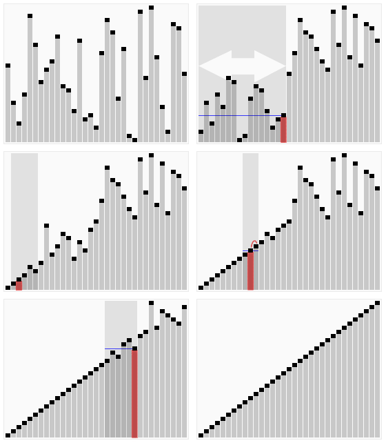
Quicksort is one of the most widespread sorting algorithms, and was the default sorting approach in Unix, C, and Java for some time. It has been replaced by fancier sorts with better real-world runtimes, but remains very effective in practice. The idea behind its implementation is to choose a “pivot” element from the collection at random, and push everything less than the pivot to its left, and everything greater than the pivot to its right. Then, simply recurse on the left and right sub-collections (the pivot is in its final sorted place).
func QuickSort(data sort.Interface, a, b int) {
    if b-a < 2 {
        return
    }

    pivot := b - 1
    finalPivotSpot := a
    for i := a; i < b; i++ {
        if data.Less(i, pivot) {
            data.Swap(i, finalPivotSpot)
            finalPivotSpot++
        }
    }
    data.Swap(finalPivotSpot, pivot)
    QuickSort(data, a, finalPivotSpot)
    QuickSort(data, finalPivotSpot+1, b)
}
Quicksort’s performance characteristics are interesting in the sense that
it has a worst case asymptotic runtime of O(n^2),
but in practice (on average),
it operates in O(nlogn) time.
It’s worst case runtime comes from the fact that
it is possible to construct an input such that the smallest (or largest) collection element
is used as a pivot on each recurrence of the algorithm.
In such a case, quicksort effectively devolves into a selection sort.
Barring that very rare situation,
quicksort performs better than other O(nlogn) algorithms
because of implementation details leading to
better cache locality, and other, non-asymptotically relevant performance benefits.
The Fancier Sorts
The fancier sorts I have alluded to are hybrid algorithms like Timsort and Introsort. The general idea of this class of sorting algorithm is that asymptotic complexity, while important, is not the only factor determining the speed of a sorting algorithm in real world workflows. Different algorithms are optimal in different scenarios, and we can take advantage of that knowledge by choosing the most efficient operations given relevant characteristics of the input data. For example, simple sorts like insertion sort perform better than more complex sorts when dealing with small datasets. As the data size grows, quicksort may become the best option. Once a certain call stack level is reached, it may make sense to switch again to something like merge sort, and so on.
A perspicuous example of hybrid sorting algorithms in practice is the default sort in Go. For a fascinating historical perspective, here’s the inventor of Timsort, Tim Peters’ original paper describing his sort implementation, which went on to be the standard sorting algorithm in Python, Java, and many other standard libraries.
Non-Comparison Based Sorts
I said earlier that all general purpose sorting algorithms are comparison based. If, however, restrictions are placed on the input, it is possible to sort without comparisons. Additionally, non-comparative sorts have the potential to achieve better optimal run time efficiencies.
A common type of non-comparative sort is Radix Sort. Loosely, this sorting algorithm works by making a single pass through the input collection, and putting its elements into pre-ordered buckets. The reason this technique doesn’t work on arbitrary input is that the buckets must be created before running the sort, and so the input data must be restricted in some way such that it is known a priori how many buckets to create.
In spite of this restriction, these sorts are useful in many situations.
For example, imagine wanting to sort a large collection of people objects based on their age (in years).
Typical intuition would say that the best option would have O(nlogn) asymptotic time complexity.
If, however, it’s reasonable to assume that ages are restricted from 0 to 250 years,
the sort can be accomplished in what is effectively O(n) time using a bucket sorting methodology.
Specifically, create an ageBuckets array with a length of 250 – a bucket for each year.
Then, iterate through the input collection,
putting each person into the bucket corresponding to their age.
This method takes O(n) time for the sort,
and another O(n) to create a sorted collection from the buckets.
Technically, because we are examining the value of each element,
the real running time is O(kn), where k is the size (length of the representation) of the values,
and for arbitrarily large values, k can grow to be of log(n) size,
so it can be argued that the real asymptotic complexity of a bucketing sort is still O(nlogn),
but we’ll leave that particular exploration for another post.
For most cases where it is practical, a bucketing sort is a nice speed win, with the tradeoff of additional memory usage.
The source code (along with tests) for the sorting algorithms presented here can be found on Github.